The distribution of tropospheric ozone (O3) globally depends on the emission of precursors (e.g., NOx), chemistry, and transport. In this study, we quantify the response of radiative forcing over 20- and 100-year time scales, to O3 and methane (CH4) perturbations caused by a marginal increase (0.1 Tg N) in anthropogenic emissions of NOx in January and July from 21 (10° × 10° grid) geographical locations in North America. Changes in the perturbations have been calculated with the global climate-chemistry transport model STOCHEM. Addition of NOx emissions led to an initial increase in global O3 burdens up to 0.9 Tg, which decayed after 4 months. Global CH4 burdens decreased (by increasing OH) by up to –0.7 Tg and decayed gradually after 6 months. Global radiative forcings resulting from the regional emission increases were calculated, accounting for changes in both O3 (using an offline radiation code) and CH4 (using a simple conversion of 0.37 mW m⁻² ppb⁻1, assuming that CH4 is well mixed in the atmosphere). Our results revealed that O3-induced time-integrated radiative forcings exhibit both positive (initial) and negative (long-term) phases in the two (20- and 100-year) time horizons. For the positive phase, both the 20- and 100-year time periods peaked at 0.454 mW m⁻² yr; however, for the negative phase, the 20-year peaked at –0.246 mW m⁻² yr and the 100-year peaked at –0.300 mW m⁻² yr. CH4, on the other hand, showed a single negative phase which peaked at –1.070 mW m⁻² yr for the 20-year time period and –1.302 mW m⁻² yr for the 100-year time period. The total net radiative forcings (assuming a linear additive for relatively small perturbations) of the CH4 term and the two O3 terms over a 100-year time period from all 21 locations produce a net climate cooling effect (negative forcings), irrespective of the season of the emission pulses. However, over a 20-year time period in winter, some emission pulses at low latitudes produce a net climate warming effect (positive forcings). Both the O3 and CH4 burdens and the associated radiative forcings depend strongly on the geographical location as well as the season of the emission pulses. They are most sensitive to emissions from low latitudes and least sensitive to emissions from mid-latitudes and high latitudes.
| Published in | International Journal of Atmospheric and Oceanic Sciences (Volume 10, Issue 1) |
| DOI | 10.11648/j.ijaos.20261001.11 |
| Page(s) | 1-12 |
| Creative Commons |
This is an Open Access article, distributed under the terms of the Creative Commons Attribution 4.0 International License (http://creativecommons.org/licenses/by/4.0/), which permits unrestricted use, distribution and reproduction in any medium or format, provided the original work is properly cited. |
| Copyright |
Copyright © The Author(s), 2026. Published by Science Publishing Group |
Radiative Forcing, Ozone, Methane, Chemistry Transport Model, Climate Model, Nitrogen Oxides, Lagrangian Model
Region | D-CH4 ppbv yr | D-O3 (short) ppbv yr | D-O3 (long) ppbv yr |
|---|---|---|---|
Washington | -0.412, -0.637 | 0.012, 0.005 | -0.002, -0.002 |
Idaho | -0.227, -0.681 | 0.007, 0.007 | -0.001, -0.003 |
Montana | -0.211, -0.743 | 0.006, 0.007 | -0.001, -0.003 |
Minnesota | -0.229, -0.658 | 0.007, 0.007 | -0.001, -0.003 |
Ontario | -0.203, -0.715 | 0.006, 0.008 | -0.001, -0.003 |
Quebec | -0.285, -0.733 | 0.008, 0.009 | -0.001, -0.003 |
New Brunswick | -0.447, -0.862 | 0.013, 0.011 | -0.002, -0.003 |
Newfoundland | -0.522, -0.893 | 0.014, 0.010 | -0.002, -0.003 |
California | -0.544, -1.153 | 0.013, 0.006 | -0.002, -0.004 |
Nevada | -0.222, -0.723 | 0.005, 0.006 | -0.001, -0.003 |
Colorado | -0.202, -0.933 | 0.006, 0.007 | -0.001, -0.004 |
Kansas | -0.270, -0.530 | 0.008, 0.004 | -0.001, -0.002 |
Kentucky | -0.316, -0.636 | 0.009, 0.006 | -0.001, -0.002 |
Washington DC | -0.456, -0.811 | 0.012, 0.007 | -0.002, -0.003 |
Mexico 1 | -0.653, -1.206 | 0.005, 0.005 | -0.003, -0.005 |
Mexico 2 | -0.279, -1.626 | 0.006, 0.009 | -0.001, -0.006 |
Texas | -0.430, -1.086 | 0.011, 0.006 | -0.002, -0.004 |
Florida | -0.623, -1.051 | 0.015, 0.006 | -0.002, -0.004 |
Mexico 3 | -1.159, -2.893 | 0.010, 0.014 | -0.004, -0.011 |
Mexico 4 | -0.802, -2.545 | 0.008, 0.014 | -0.003, -0.010 |
Honduras | -0.999, -2.582 | 0.012, 0.014 | -0.004, -0.010 |
Region | D-CH4 ppbv yr | D-O3 (short) ppbv yr | D-O3 (long) ppbv yr |
|---|---|---|---|
Washington | -0.502, -0.775 | 0.012, 0.005 | -0.002, -0.003 |
Idaho | -0.277, -0.828 | 0.007, 0.007 | -0.001, -0.003 |
Montana | -0.257, -0.904 | 0.006, 0.007 | -0.001, -0.003 |
Minnesota | -0.278, -0.801 | 0.007, 0.007 | -0.001, -0.003 |
Ontario | -0.247, -0.871 | 0.006, 0.008 | -0.001, -0.003 |
Quebec | -0.347, -0.892 | 0.008, 0.009 | -0.001, -0.003 |
New Brunswick | -0.544, -1.049 | 0.013, 0.011 | -0.002, -0.004 |
Newfoundland | -0.635, -1.087 | 0.014, 0.010 | -0.002, -0.004 |
California | -0.662, -1.403 | 0.013, 0.006 | -0.003, -0.005 |
Nevada | -0.270, -0.880 | 0.005, 0.006 | -0.001, -0.003 |
Colorado | -0.246, -1.135 | 0.006, 0.007 | -0.001, -0.004 |
Kansas | -0.329, -0.645 | 0.008, 0.004 | -0.001, -0.002 |
Kentucky | -0.384, -0.774 | 0.009, 0.006 | -0.001, -0.003 |
Washington DC | -0.554, -0.987 | 0.012, 0.007 | -0.002, -0.004 |
Mexico 1 | -0.794, -1.468 | 0.005, 0.005 | -0.003, -0.006 |
Mexico 2 | -0.339, -1.978 | 0.006, 0.009 | -0.001, -0.008 |
Texas | -0.523, -1.322 | 0.011, 0.006 | -0.002, -0.005 |
Florida | -0.758, -1.279 | 0.015, 0.006 | -0.003, -0.005 |
Mexico 3 | -1.409, -3.520 | 0.010, 0.014 | -0.005, -0.014 |
Mexico 4 | -0.975, -3.097 | 0.008, 0.014 | -0.004, -0.012 |
Honduras | -1.214, -3.143 | 0.012, 0.014 | -0.005, -0.012 |
O3 | Ozone |
NOx & NOy | Nitrogen Oxides |
CH4 | Methane |
OH | Hydroxyl Radical |
Tg | Teragram |
IPCC | Intergovernmental Panel on Climate Change |
CO | Carbon Monoxide |
SO2 | Sulfur Dioxide |
H2 | Hydrogen |
UV | Ultraviolet |
VOC | Volatile Organic Compounds |
IIASA | International Institute for Applied Systems Analysis |
NASA | National Aeronautics and Space Administration |
EDGAR | Emissions Database for Global Atmospheric Research |
ppbv | Parts Per Billion by Volume |
| [1] | IPCC. (2001). Climate Change 2001: The Scientific Basis. Contribution of Working Group I to the Third Assessment Report of the Intergovernmental Panel on Climate Change (J. T. Houghton, Y. Ding, D. J. Griggs, M. Noguer, P. J. van der Linden, X. Dai, K. Maskell, & C. A. Johnson, Eds.). Cambridge University Press. |
| [2] | Fuglestvedt, J. S., Berntsen, T. K., Godal, O., & Skodvin, T. (1999). Climate implications of GWP-based reductions in greenhouse gas emissions. Geophysical Research Letters, 26(6), 739-742. |
| [3] | Wild, O., & Prather, M. J. (2000). Excitation of the primary tropospheric chemical mode in a global three-dimensional model. Journal of Geophysical Research: Atmospheres, 105(D20), 24647-24660. |
| [4] | Derwent, R. G., Collins, W. J., Johnson, C. E., & Stevenson, D. S. (2001). Transient behaviour of tropospheric ozone precursors in a global 3-D CTM and their indirect greenhouse effects. Climatic Change, 49(4), 463-487. |
| [5] | Isaksen, I. S. A., Hov, Ø., & Hesstvedt, E. (1978). Ozone generation over rural areas. Environmental Science & Technology, 12(11), 1279-1283. |
| [6] | Lin, X., Trainer, M., & Liu, S. C. (1988). On the nonlinearity of the tropospheric ozone production. Journal of Geophysical Research: Atmospheres, 93(D12), 15879-15888. |
| [7] | Berntsen, T. K., Fuglestvedt, J. S., Joshi, M. M., Shine, K. P., Stuber, N., Ponater, M. & Li, L. (2005). Response of climate to regional emissions of ozone precursors: Sensitivities and warming potentials. Tellus B: Chemical and Physical Meteorology, 57(4), 283-304. |
| [8] | Wang, W. C., & Sze, N. D. (1980). Coupled effects of atmospheric N2O and O3 on the Earth's climate. Nature, 286(5774), 589-590. |
| [9] | Lacis, A. A., Wuebbles, D. J., & Logan, J. A. (1990). Radiative forcing of climate by changes in the vertical distribution of ozone. Journal of Geophysical Research: Atmospheres, 95(D7), 9971-9981. |
| [10] | Berntsen, T. K., Karlsdottir, S., & Jaffe, D. A. (1997). Influence of Asian emissions on the composition of air reaching the North American west coast. Geophysical Research Letters, 24(23), 3113-3116. |
| [11] | Stevenson, D. S., R. M. Doherty, M. G. Sanderson, W. J. Collins, C. E. Johnson, and R. G. Derwent (2004), Radiative forcing from aircraft NOx emissions: Mechanisms and seasonal dependence, J. Geophys. Res., 109, D17307, |
| [12] | Collins, W. J., Stevenson, D. S., Johnson, C. E., & Derwent, R. G. (1997). Tropospheric ozone in a global-scale three-dimensional Lagrangian model and its response to NOx emission controls. Journal of Atmospheric Chemistry, 26(3), 223-274. |
| [13] | Maryon, R. H., & Best, M. J. (1992). The NAME 4-day mesoscale atmospheric dispersion model: Description and validation against ETEX data. UK Met Office Turbulence and Diffusion Note, 227. |
| [14] | Li, D., & Shine, K. P. (1995). A 4-D ozone climatology for UGAMP models. UGAMP Internal Report, 35, 1-35. University of Reading. |
| [15] | Murphy, D. M., & Fahey, D. W. (1994). An estimate of the flux of stratospheric reactive nitrogen and ozone into the troposphere. Journal of Geophysical Research: Atmospheres, 99(D3), 5325-5332. |
| [16] | Dentener, F., Kinne, S., Bond, T., Boucher, O., Cofala, J., Generoso, S. & Van Aardenne, J. (2005). Emissions of primary aerosol and precursor gases in the years 2000 and 1750 prescribed data-sets for AeroCom. Atmospheric Chemistry and Physics Discussions, 5(3), 3589-3629. |
| [17] | Olivier, J. G. J., & Berdowski, J. J. M. (2001). Global emissions sources and sinks. In J. Berdowski, R. Guicherit, & B. J. Heij (Eds.), The Climate System (pp. 33-78). A. A. Balkema Publishers. |
| [18] | Wild, O., Prather, M. J., & Akimoto, H. (2001). Indirect long-term global radiative cooling from NOx emissions. Geophysical Research Letters, 28(9), 1719-1722. |
| [19] | Schimel, D., Alves, D., Enting, I., Heimann, M., Joos, F., Raynaud, D.,.. & Wigley, T. (1996). CO2 and the carbon cycle. In Climate Change 1995: The Science of Climate Change (pp. 65-131). Cambridge University Press. |
| [20] | Naik, V., Mauzerall, D., Horowitz, L., Schwarzkopf, M. D., Ramaswamy, V., & Oppenheimer, M. (2005). Net radiative forcing due to changes in regional emissions of tropospheric ozone precursors. Journal of Geophysical Research: Atmospheres, 110(D24), D24306. |
| [21] | Derwent, R. G., Stevenson, D. S., Collins, W. J., & Johnson, C. E. (2006). Intercontinental transport and the impacts of anthropogenic pollutants on air quality and climate. Atmospheric Environment, 40(22), 4049-4052. |
| [22] | IPCC, 2023: Summary for Policymakers. In: Climate Change 2023: Synthesis Report. Contribution of Working Groups I, II and III to the Sixth Assessment Report of the Intergovernmental Panel on Climate Change [Core Writing Team, H. Lee and J. Romero (eds.)]. IPCC, Geneva, Switzerland, pp. 1-34, |
| [23] | Collins, W. J., Derwent, R. G., Johnson, C. E., & Stevenson, D. S. (2002). The oxidation of organic compounds and their fluxes in the troposphere. Journal of Geophysical Research: Atmospheres, 107(D16), ACH 9-1-ACH 9-8. |
| [24] | Khan, M. A. H., M. E. Jenkin, A. Foulds, R. G. Derwent, C. J. Percival, and D. E. Shallcross (2017), A modeling study of secondary organic aerosol formation from sesquiterpenes using the STOCHEM global chemistry and transport model, J. Geophys. Res. Atmos., 122, 4426-4439, |
| [25] | Johnson, CE, Stevenson, DS, Collins, WJ & Derwent, RG 2002, 'Interannual variability in methane growth rate simulated with a coupled Ocean-Atmosphere-Chemistry model' Geophysical Research Letters, vol 29, no. 19, pp. 1-4., |
| [26] | Khan, M. A. H., Lyons, K., Chhantyal-Pun, R., McGillen, M. R., Caravan, R. L., Taatjes, C. A., et al. (2018). Investigating the tropospheric chemistry of acetic acid using the global 3-D chemistry transport model, STOCHEM-CRI. Journal of Geophysical Research: Atmospheres, 123, 6267-6281. |
| [27] | P. Cristofanelli, P. Bonasoni, W. Collins, J. Feichter, C. Forster, P. James, A. Kentarchos, P. W. Kubik, C. Land, J. Meloen, G. J. Roelofs, P. Siegmund, M. Sprenger, C. Schnabel, A. Stohl, L. Tobler, L. Tositti, T. Trickl, P. Zanis (2003), Stratosphere-to-troposphere transport: A model and method evaluation, J. Geophys. Res., 108, 8525, |
| [28] | Stevenson, D. S., Collins, W. J., Johnson, C. E. and Derwent, R. G. (1998), Intercomparison and evaluation of atmospheric transport in a Lagrangian model (STOCHEM), and an Eulerian model (UM), using 222Rn as a short-lived tracer. Q. J. R. Meteorol. Soc., 124: 2477-2491. |
| [29] | W. J Collins, D. S Stevenson, C. E Johnson, R. G Derwent, The European regional ozone distribution and its links with the global scale for the years 1992 and 2015, Atmospheric Environment, Vol. 34,, 2000, 255-267, |
| [30] | Collins, W. J., D. S. Stevenson, C. E. Johnson, and R. G. Derwent (1999), Role of convection in determining the budget of odd hydrogen in the upper troposphere, J. Geophys. Res., 104(D21), 26927-26941, |
APA Style
Damoah, R. (2026). Time Integrated Radiative Forcing from North American NOX Emissions: Climate Effect over 20- and 100-year Time Scales. International Journal of Atmospheric and Oceanic Sciences, 10(1), 1-12. https://doi.org/10.11648/j.ijaos.20261001.11
ACS Style
Damoah, R. Time Integrated Radiative Forcing from North American NOX Emissions: Climate Effect over 20- and 100-year Time Scales. Int. J. Atmos. Oceanic Sci. 2026, 10(1), 1-12. doi: 10.11648/j.ijaos.20261001.11
@article{10.11648/j.ijaos.20261001.11,
  author = {Richard Damoah},
  title = {Time Integrated Radiative Forcing from North American NOX Emissions: Climate Effect over 20- and 100-year Time Scales},
  journal = {International Journal of Atmospheric and Oceanic Sciences},
  volume = {10},
  number = {1},
  pages = {1-12},
  doi = {10.11648/j.ijaos.20261001.11},
  url = {https://doi.org/10.11648/j.ijaos.20261001.11},
  eprint = {https://article.sciencepublishinggroup.com/pdf/10.11648.j.ijaos.20261001.11},
  abstract = {The distribution of tropospheric ozone (O3) globally depends on the emission of precursors (e.g., NOx), chemistry, and transport. In this study, we quantify the response of radiative forcing over 20- and 100-year time scales, to O3 and methane (CH4) perturbations caused by a marginal increase (0.1 Tg N) in anthropogenic emissions of NOx in January and July from 21 (10° × 10° grid) geographical locations in North America. Changes in the perturbations have been calculated with the global climate-chemistry transport model STOCHEM. Addition of NOx emissions led to an initial increase in global O3 burdens up to 0.9 Tg, which decayed after 4 months. Global CH4 burdens decreased (by increasing OH) by up to –0.7 Tg and decayed gradually after 6 months. Global radiative forcings resulting from the regional emission increases were calculated, accounting for changes in both O3 (using an offline radiation code) and CH4 (using a simple conversion of 0.37 mW m⁻² ppb⁻1, assuming that CH4 is well mixed in the atmosphere). Our results revealed that O3-induced time-integrated radiative forcings exhibit both positive (initial) and negative (long-term) phases in the two (20- and 100-year) time horizons. For the positive phase, both the 20- and 100-year time periods peaked at 0.454 mW m⁻² yr; however, for the negative phase, the 20-year peaked at –0.246 mW m⁻² yr and the 100-year peaked at –0.300 mW m⁻² yr. CH4, on the other hand, showed a single negative phase which peaked at –1.070 mW m⁻² yr for the 20-year time period and –1.302 mW m⁻² yr for the 100-year time period. The total net radiative forcings (assuming a linear additive for relatively small perturbations) of the CH4 term and the two O3 terms over a 100-year time period from all 21 locations produce a net climate cooling effect (negative forcings), irrespective of the season of the emission pulses. However, over a 20-year time period in winter, some emission pulses at low latitudes produce a net climate warming effect (positive forcings). Both the O3 and CH4 burdens and the associated radiative forcings depend strongly on the geographical location as well as the season of the emission pulses. They are most sensitive to emissions from low latitudes and least sensitive to emissions from mid-latitudes and high latitudes.},
 year = {2026}
}
TY  - JOUR
T1  - Time Integrated Radiative Forcing from North American NOX Emissions: Climate Effect over 20- and 100-year Time Scales
AU  - Richard Damoah
Y1  - 2026/03/30
PY  - 2026
N1  - https://doi.org/10.11648/j.ijaos.20261001.11
DO  - 10.11648/j.ijaos.20261001.11
T2  - International Journal of Atmospheric and Oceanic Sciences
JF  - International Journal of Atmospheric and Oceanic Sciences
JO  - International Journal of Atmospheric and Oceanic Sciences
SP  - 1
EP  - 12
PB  - Science Publishing Group
SN  - 2640-1150
UR  - https://doi.org/10.11648/j.ijaos.20261001.11
AB  - The distribution of tropospheric ozone (O3) globally depends on the emission of precursors (e.g., NOx), chemistry, and transport. In this study, we quantify the response of radiative forcing over 20- and 100-year time scales, to O3 and methane (CH4) perturbations caused by a marginal increase (0.1 Tg N) in anthropogenic emissions of NOx in January and July from 21 (10° × 10° grid) geographical locations in North America. Changes in the perturbations have been calculated with the global climate-chemistry transport model STOCHEM. Addition of NOx emissions led to an initial increase in global O3 burdens up to 0.9 Tg, which decayed after 4 months. Global CH4 burdens decreased (by increasing OH) by up to –0.7 Tg and decayed gradually after 6 months. Global radiative forcings resulting from the regional emission increases were calculated, accounting for changes in both O3 (using an offline radiation code) and CH4 (using a simple conversion of 0.37 mW m⁻² ppb⁻1, assuming that CH4 is well mixed in the atmosphere). Our results revealed that O3-induced time-integrated radiative forcings exhibit both positive (initial) and negative (long-term) phases in the two (20- and 100-year) time horizons. For the positive phase, both the 20- and 100-year time periods peaked at 0.454 mW m⁻² yr; however, for the negative phase, the 20-year peaked at –0.246 mW m⁻² yr and the 100-year peaked at –0.300 mW m⁻² yr. CH4, on the other hand, showed a single negative phase which peaked at –1.070 mW m⁻² yr for the 20-year time period and –1.302 mW m⁻² yr for the 100-year time period. The total net radiative forcings (assuming a linear additive for relatively small perturbations) of the CH4 term and the two O3 terms over a 100-year time period from all 21 locations produce a net climate cooling effect (negative forcings), irrespective of the season of the emission pulses. However, over a 20-year time period in winter, some emission pulses at low latitudes produce a net climate warming effect (positive forcings). Both the O3 and CH4 burdens and the associated radiative forcings depend strongly on the geographical location as well as the season of the emission pulses. They are most sensitive to emissions from low latitudes and least sensitive to emissions from mid-latitudes and high latitudes.
VL  - 10
IS  - 1
ER  -
Climate Science Division, Morgan State University, Baltimore, United States
Biography: Richard Damoah is Assistant Professor in the Climate Science Division at Morgan State, International Research Associate at the Latin American Technical University in El Salvador and the Director of All Nations University Space Systems Technology Laboratory in Ghana. He has more than 20 years’ experience in chemistry climate modeling, radiative transfer modeling, trajectory modeling, pollution measurement and data analysis with strong programming skills. Before joining Morgan Dr. Damoah had worked at (1) NASA Goddard Space Flight Center in Maryland as Associate Research Scientist under the GESTAR program, (2) University of Waterloo in Ontario, Canada as Research Fellow and (3) University of Edinburgh in UK as a Postdoc. Dr Damoah graduated with Bsc in Physics at University of Cape-Coast in Ghana, Msc in Environmental Physics at University of Bremen in Germany and PhD in Natural Sciences specializing in Air Pollution Transport Modeling, at Technical University of Munich also in Germany.
Research Fields: Air Quality, Climate Change, Climate Modeling, Climate and Public Health, Atmospheric Pollution, Air Pollution Transport, Atmospheric Trajectory Modeling

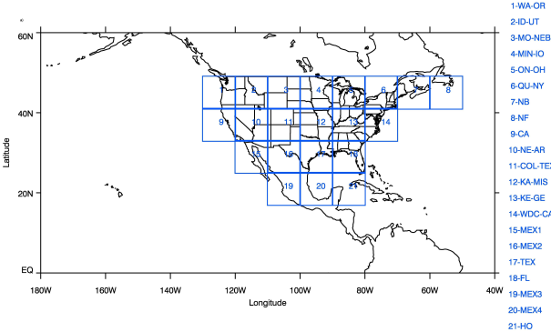
Figure 1. Map of North America showing all the 21 10° × 10° grid emission locations.
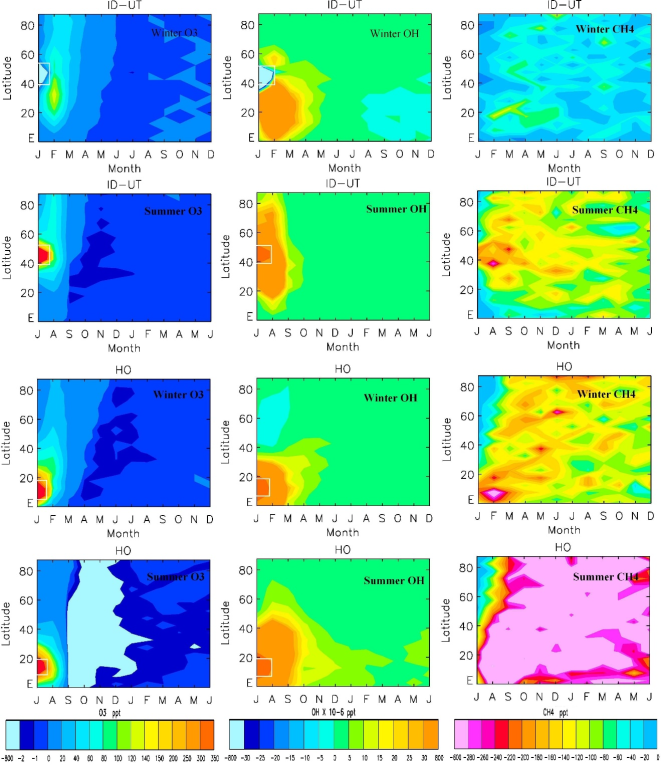
Figure 2. Time development of monthly mean O3 (left column), OH (middle column), and CH4 (right column) anomalies. The first two rows from the top are for Idaho pulses in January and July, and the last two rows are for Honduras emission pulses. The white rectangles show the locations of the emission pulses.
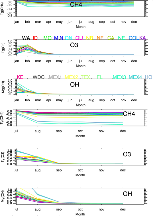
Figure 3. Time development of global CH4, O3, and OH anomalies due to the NOx emission pulses. The colors show the various locations of the pulses, ranging from Washington to Honduras. The first three panels from the top are CH4, O3, and OH anomalies for winter pulses, and the bottom three panels are for summer pulses.
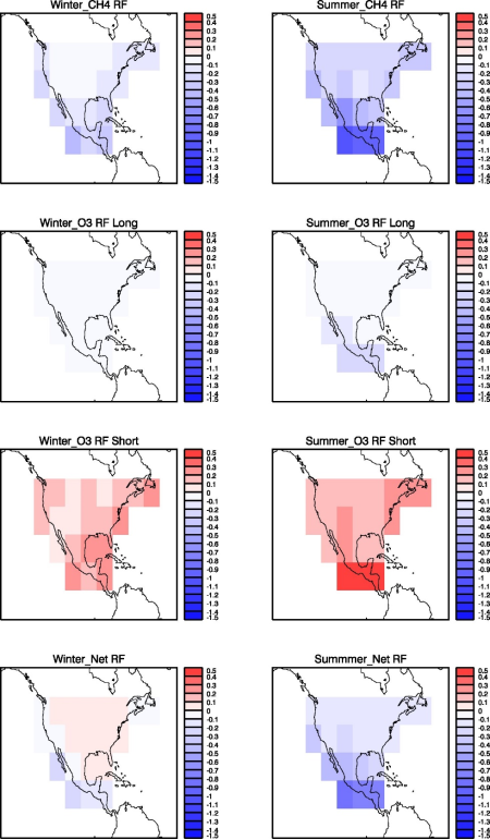
Figure 4. 20-year time-integrated radiative forcing (in mW m-2 yr) due to CH4 (first row), O3 long-term (second row), O3 short-term (third row), and total net (fourth row) responses to NOx emission pulses emitted at all 21 locations in winter (left column) and summer (right column) seasons.
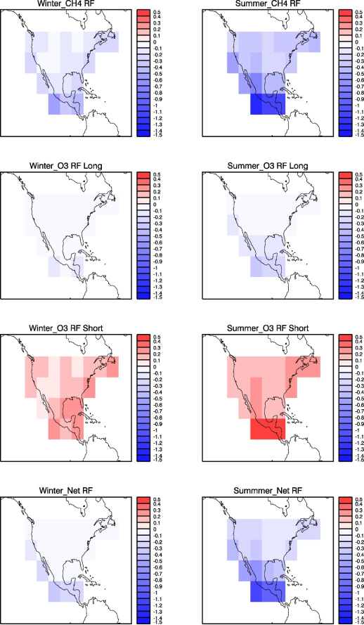
Figure 5. 100-year time-integrated radiative forcing (in mW m-2 yr) due to CH4 (first row), O3 long-term (second row), O3 short-term (third row), and total net (fourth row) responses to NOx emission pulses emitted at all 21 locations in winter (left column) and summer (right column) seasons.